How to Insert Arrow in Google Sheets

Arrows are one of the most underrated tools in Google Sheets. They can make your spreadsheets easier to read, highlight important data, and even guide users through dashboards or workflows.

In this guide, we’ll cover everything about how to insert arrow in Google Sheets—from simple symbols to custom arrow shapes and even using them for data visualization.

How to Insert Arrow in Google Sheets

There are several ways to insert arrow in Google Sheets. You can use the Drawing tool, copy special characters, or even insert arrows automatically with formulas. Let’s explore each method step by step.

Drawing Arrows in Google Sheets

1. Open your Google Sheets document.
2. Click on the cell where you want the arrow to appear.
3. Click on the “Insert” options from the “Menu bar”.
4. Hover your mouse over “Drawing”.
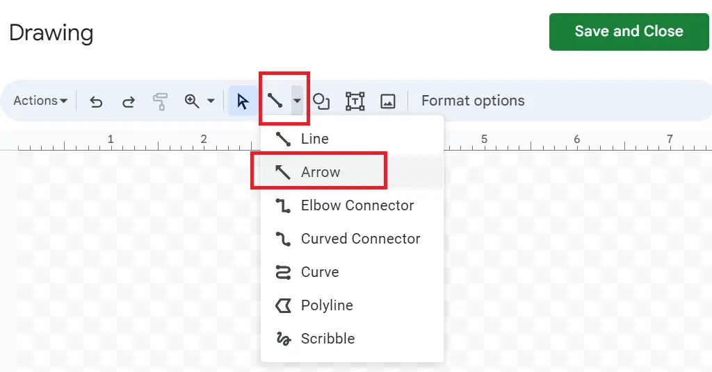
5. Select the arrow shape from the “Toolbar”.
6. Click and drag on the drawing canvas to create the arrow.

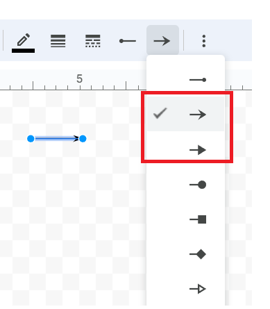
Once the arrow is drawn, you can customize it by changing the line color, thickness, arrowhead style, or even switching to curved and double arrows.

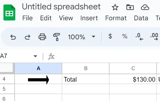
When you’re happy with the result, click Save and Close. The arrow will now appear in your Google Sheet where you selected it.

This method is perfect if you want to insert arrow in Google Sheets including curved arrows, double arrows, and directional arrows.

Insert Arrow in Google Sheets Using Special Characters

Another simple method to insert arrow in Google Sheets is by using the Special Characters option in Google Docs. While Sheets doesn’t have a built-in character picker, you can copy arrows from Docs and paste them directly into your spreadsheet.

1. Open a Google Docs document.
2. From the top menu, click Insert → Special Characters.
3. In the search box, type arrow.
4. You’ll see a wide range of arrow options, including up arrows (↑), down arrows (↓), left/right arrows (← →), curved arrows, and double arrows (⇐ ⇒).
5. Click on the arrow you want—it will be inserted into your Google Doc.
6. Simply copy the arrow from Google Docs and paste it into a Google Sheets cell.

Using the CHAR Function for Arrows

You can also insert arrow in Google Sheets automatically with the CHAR() function. This is especially useful when you want arrows to update dynamically based on data changes.

The CHAR() function returns a character based on its Unicode number. Since arrows are part of the Unicode character set, you can insert them directly into your cells using this formula.

• =CHAR(8593) → ↑ (Up arrow)
• =CHAR(8595) → ↓ (Down arrow)
• =CHAR(8592) → ← (Left arrow)
• =CHAR(8594) → → (Right arrow)

Using Arrows for Data Visualization

Instead of showing plain numbers, arrows act as visual indicators that make it much easier for readers to spot trends, changes, or key points in your data.

a) Trend Arrows with Formulas

One of the most common uses for arrows is to show whether data is increasing, decreasing, or staying the same. Instead of expecting someone to read through numbers line by line, you can instantly communicate direction with an arrow

=IF(B2>A2,"↑",IF(B2<A2,"↓","→"))

How it works:

• ↑ Upward arrow → the data increased.
• ↓ Downward arrow → the data decreased.
• → Side arrow → no change.

b) Arrow Annotations in Charts

If you’re building a dashboard or presentation, you might want arrows directly inside a chart to point at important trends.

1. Create your chart in Google Sheets.
2. Go to the Insert > Drawing > New tool.
3. Draw an arrow shape (straight, curved, or double arrow).
4. Place the arrow in the chart area to highlight an important data point or trend.
5. Customize the style, thickness, and color of the arrow so it stands out.

This method works great for highlighting key data points, directional changes, or important trends.

Whether you use the Drawing tool, copy special characters, or rely on formulas, knowing how to insert arrow in Google Sheets makes your spreadsheets more visual, interactive, and easy to understand.